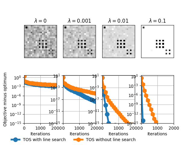
Estimating a sparse and low rank matrix

Out:

#features 400
beta = 0
beta = 0.001
beta = 0.01
Achieved relative tolerance at iteration 806
Achieved relative tolerance at iteration 2140
beta = 0.1
Achieved relative tolerance at iteration 147
Achieved relative tolerance at iteration 942

import numpy as np
from scipy.sparse import linalg as splinalg
import pylab as plt
import copt as cp

# .. Generate synthetic data ..
np.random.seed(1)

sigma_2 = 0.6
N = 100
d = 20
blocks = np.array([2 * d /10,1 * d /10,1 * d /10,3 * d /10,3 * d / 10]).astype(np.int)
epsilon = 10**(-15)

mu = np.zeros(d)
Sigma = np.zeros((d,d))
blck = 0
for k in range(len(blocks)):
    v = 2 * np.random.rand(int(blocks[k]),1)
    v = v * (abs(v) > 0.9)
    Sigma[blck:blck+blocks[k],blck:blck+blocks[k]] = np.dot(v, v.T)
    blck = blck + blocks[k]
X = np.random.multivariate_normal(mu, Sigma + epsilon * np.eye(d) ,N) + sigma_2 * np.random.randn(N,d);
Sigma_hat = np.cov(X.T)

threshold = 1e-5
Sigma[np.abs(Sigma) < threshold] = 0
Sigma[np.abs(Sigma) >= threshold] = 1

# .. generate some data ..

max_iter = 5000

n_features = np.multiply(*Sigma.shape)
n_samples = n_features
print('#features', n_features)
A = np.random.randn(n_samples, n_features)

sigma = 1.
b = A.dot(Sigma.ravel()) + sigma * np.random.randn(n_samples)

# .. compute the step-size ..
s = splinalg.svds(A, k=1, return_singular_vectors=False,
                  tol=1e-3, maxiter=500)[0]
step_size = 1. / cp.utils.get_lipschitz(A, 'square')
f = cp.utils.HuberLoss(A, b)

# .. run the solver for different values ..
# .. of the regularization parameter beta ..
all_betas = [0, 1e-3, 1e-2, 1e-1]
all_trace_ls, all_trace_nols, all_trace_pdhg_nols, all_trace_pdhg = [], [], [], []
all_trace_ls_time, all_trace_nols_time, all_trace_pdhg_nols_time, all_trace_pdhg_time = [], [], [], []
out_img = []
for i, beta in enumerate(all_betas):
    print('beta = %s' % beta)
    G1 = cp.utils.NuclearNorm(beta, *Sigma.shape)
    G2 = cp.utils.L1Norm(beta)

    def loss(x):
        return f(x) + G1(x) + G2(x)

    cb_tosls = cp.utils.Trace()
    x0 = np.zeros(n_features)
    cb_tosls(x0)
    tos_ls = cp.minimize_TOS(
        f.func_grad, x0, G2.prox, G1.prox, step_size=5 * step_size,
        max_iter=max_iter, tol=1e-14, verbose=1,
        callback=cb_tosls, h_Lipschitz=beta)
    trace_ls = np.array([loss(x) for x in cb_tosls.trace_x])
    all_trace_ls.append(trace_ls)
    all_trace_ls_time.append(cb_tosls.trace_time)

    cb_tos = cp.utils.Trace()
    x0 = np.zeros(n_features)
    cb_tos(x0)
    tos = cp.minimize_TOS(
        f.func_grad, x0, G1.prox, G2.prox,
        step_size=step_size,
        max_iter=max_iter, tol=1e-14, verbose=1,
        line_search=False, callback=cb_tos)
    trace_nols = np.array([loss(x) for x in cb_tos.trace_x])
    all_trace_nols.append(trace_nols)
    all_trace_nols_time.append(cb_tos.trace_time)
    out_img.append(tos.x)

# .. plot the results ..
f, ax = plt.subplots(2, 4, sharey=False)
xlim = [0.02, 0.02, 0.1]
for i, beta in enumerate(all_betas):
    ax[0, i].set_title(r'$\lambda=%s$' % beta)
    ax[0, i].set_title(r'$\lambda=%s$' % beta)
    ax[0, i].imshow(out_img[i].reshape(Sigma.shape),
                    interpolation='nearest', cmap=plt.cm.gray_r)
    ax[0, i].set_xticks(())
    ax[0, i].set_yticks(())

    fmin = min(np.min(all_trace_ls[i]), np.min(all_trace_nols[i]))
    plot_tos, = ax[1, i].plot(
        all_trace_ls[i] - fmin,
        lw=4, marker='o', markevery=100,
        markersize=10)

    plot_nols, = ax[1, i].plot(
        all_trace_nols[i] - fmin,
        lw=4, marker='h', markevery=100,
        markersize=10)

    ax[1, i].set_xlabel('Iterations')
    ax[1, i].set_yscale('log')
    ax[1, i].set_ylim((1e-15, None))
    ax[1, i].set_xlim((0, 2000))
    ax[1, i].grid(True)


plt.gcf().subplots_adjust(bottom=0.15)
plt.figlegend(
    (plot_tos, plot_nols),
    ('TOS with line search', 'TOS without line search'), ncol=5,
    scatterpoints=1,
    loc=(-0.00, -0.0), frameon=False,
    bbox_to_anchor=[0.05, 0.01])

ax[1, 0].set_ylabel('Objective minus optimum')
plt.show()

Total running time of the script: ( 9 minutes 17.756 seconds)